When we talk about today’s generative modelling landscape, the two main talk of the town use cases that people are interested in the most are language modelling and image generation. The most influential model architecture that enables language modelling today is, as we all know, the transformers or varients of transformers. On the otherhand, in image generation field, prominent models like stable diffusion, OpenAI’s GLIDE models or Dall-E 2 are made possible by diffusion models. Among various architectures and methods used in image generation like GAN, VAE or flow-based methods, diffusion models are still dominant to this day and is one of the most interesting models for me. Methodologies used in making the diffusion model work are very interesting and I will try to entertain you too in this article.
Before diffusion
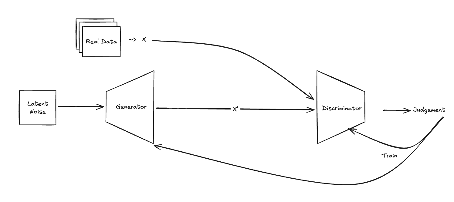
Before diffusion models came around, we had GAN and Autoencoder models. Let’s talk a little bit about them first before we go to diffusion models. Firstly, in GAN architecture, the training process consists of two models, Generator and Discriminator pitted against each other trying to outwit one another. Generator will try to fool the Discriminator by generating data samples as similar as possible to the real world data distribution while Discriminator will classify real data and fake data generated by Generator. Generator is rewarded when Discriminator incorrectly classifies its data sample and Discriminator is rewarded to correctly classify the real ones. It is an interesting and clever training method but it is quite unstable to train two models simultaneously.
GAN
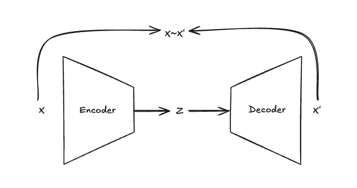
Autoencoder architecture also includes two models but they are not racing against each other; they are cooperating to create the information bottleneck to compress the input data into a lower dimensional latent representation. Encoder compresses the input data into a bottleneck latent representation and Decoder tries to reconstruct the input data from the latent. Two models end-to-end try to optimize the reconstruction loss which pushes the model to generate output as similar as possible to the input data. There are many other variations of autoencoders also, namely denoising autoencoders, VAE, beta-VAE, VQ-VAE, etc.
In VAE, the latent representation is a probability distribution instead of an exact latent variable. By making the latent representation a probability distribution, the space becomes continuous and thus enchancing the interpolation nature when generating the image. There are very interesting mechanisms enabling the VAE work, for example, minimizing the KL divergence between latent distribution and a Gaussian distribution to make the latent space to be regularized in accordance with a simple prior distribution so that similar features will overlap and different features will be separated more. I will not talk too much about VAE here as we have to dig deeper into diffusion models. If you are interested in autoencoder architectures, Lilian Weng’s From Autoencoder to Beta-VAE is very informational.
Autoencoder
Score function: the heart of diffusion
When we train diffusion models, what the diffusion model is trying to do is to estimate the score function \(\nabla_xlogp(x)\). Here, what \(\nabla_xlogp(x)\) means is model is trying to find the gradient w.r.t input x. In case of a typical neural network, we try to optimize the network using the gradient w.r.t θ, but in diffusion we will optimize the gradient of the input itself. In other words, we are trying to modify the input image to be more similar to a target image. In this case, input is a noisy and corrupted image and the target will be the clean and uncorrupted image. Or, in most of the cases, input is a noisy image and the model will predict the intensity of noise added to the clean image.
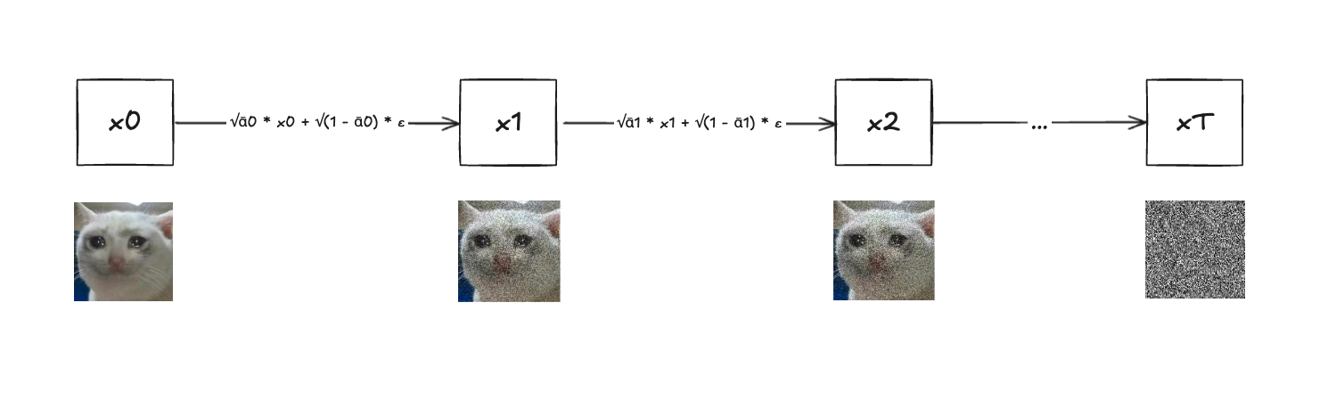
So, how do we corrupt the input image? We gradually corrupt the input image by adding additive Gaussian noises step by step. Let’s assume input image is \(x_0\) and we corrupt it T times, the final image is \(x_T\). The Gaussian nosie we add at timestep t is εt and we control the noising procedure with a variance schedule, \(\beta_t\). In this case, the noising formula at timestep t will be:
\(x_t = \sqrt{(1 - \beta_t)} . x_{t-1} + \sqrt{\beta_t} . \epsilon_{t-1}\)
What is the purpose of \(\beta_t\) here? \(\beta_t\) is a linear schedule and it gradually increases as timestep t goes. For example, \(\beta_0\) starts from 0.0001 to \(\beta_t\) ending with 0.02. What it does is it gradually increases the intensity of the noise. In above formula, we can see that we scale the \(x_{t-1}\) with (1-\(\beta_t\)) and scale the noise \(\epsilon_{t-1}\) with \(\beta_t\). The reason we do so is to prevent the \(x_t\) from exploding by reducing the intensity of the \(x_{t-1}\) before adding more noises \(\epsilon_{t-1}\).
Adding noises step by step in this manner is slow so we can apply a clever mathematical trick to add the noises directly to the \(x_0\) with the formula:
\(x_t = \sqrt{\bar{\alpha}_t} . x_{\theta} + \sqrt{(1 - \bar{\alpha}_t)} . \epsilon\)
\(\alpha_t = 1 - \beta_t\)
\(\bar{\alpha}_t = \alpha_1 . \alpha_2 . ... . \alpha_t\)
By doing so we can add the gaussian noise \(\epsilon\) to the \(x_0\) and get the \(x_t\) directly in one single step by sampling the variance \(\bar{\alpha}_t\) at timestep t. 🤯
Noising steps
Model Architecture
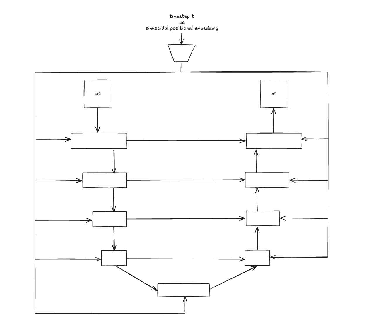
The model we use in diffusion is a simple U-net architecture which takes in a corrupted image as input and predicts the noise added. Then we can recover the clean image by subtracting the predicted noise from the corrupted image. How we do step-by-step at training time is:
- Sample an image \(x_0\) from the dataset X
- Sample the timestep t from 0<t<T
- Generate \(x_t\) by using gaussian noise \(\epsilon\) and timestep t
- Feed \(x_t\) to U-net along with timestep t (How to feed timestep t to U-net? I will explain below)
- U-net predict noise at timestep t, \(\epsilon_t\)
So, now you have the question of how does we feed timestep t to the U-net? We do it by generating sinusoidal timestep embedding vector from t and concatenate it to each of the feature vector of U-net. That way, model can make sense of the amount of noise added at timestep t by looking at \(x_t\) and sinusoidal embedding of t.
Diffusion Unet Architecture
Denoising at inference time
Now that we have trained our diffusion model to predict the noise intensity at a given timestep, how do we use that predicted noise at inference time to generate creative and interesting images? If you have ever used a diffusion model to generate images, you might have noticed that we have to give num_inference_steps parameter. At inference time, a random gaussian noise and num_inference_steps T is given as input to the model and model predict the noise \(\epsilon_t\). \(\epsilon_t\) is used to denoise \(x_t\) to get \(x_{t-1}\). This denoising process is done iteratively until we get \(x_0\). The \(\epsilon_t\) is the noise added to the clean image at timestep t, so we cannot directly use that to get \(x_{t-1}\). So what we do is:
\(x_{t-1} = \frac{1}{\sqrt{\alpha_t}} . (x_t - \frac{1-αₜ}{\sqrt{(1 - \bar{\alpha_t})}} . \epsilon_t) + \sigma_t . z\)
In the above formula, you might have noticed we have a new parameter z. That is a stochastic gaussian noise added after each denoising step to avoid stucking at a random direction along the way. Without that stochastic noise, if the model goes down the bad path and get stuck, it won’t be able to get out of that nonoptimal direction.
What does guidance do?
When we use diffusion models to generate images by giving prompts to the model, we are actually using conditional diffusion models. The model I explained in previous sections is an unconditioned model but in the case of prompting the model to generate the image that we want, we need conditioning or guidance when we train the diffusion model. That guidance is theoretically a classifier model, where an input image is classified according to a text label.
Let us assume that x is the noisy input image and y is the label or the text prompt, by using Bayes’ rule,
\(p(x\|y) = \frac{p(y\|x) . p(x)}{p(y)}\)
which means that to predict the noise intensity of x, guided by y, we need a classifier p(y|x). When we take log of the Bayes’ rule,
\(logp(x\|y) = logp(y\|x) + logp(x) − logp(y)\)
\(\nabla_xlogp(x\|y) = \nabla_xlogp(y\|x) + \nabla_xlogp(x)\)
which means that to predict the y-guided noise of x, we have to use the gradient of the classifier p(y|x) and the score function p(x). We can ignore p(y) here because when we only care for the gradient w.r.t x, p(y) becomes constant.
And we scale the guidance term in the formula with γ, which you might have already known as the guidance_scale parameter if you are familiar with huggingface’s diffusers library. The formula becomes
\(\nabla_xlogp(x\|y) = \nabla_xlogp(x) + \gamma.\nabla_xlogp(y\|x)\)
In reality, using a classifier as the guidance for the diffusion model is a bit cumbersome because we cannot just use a pretrained classifier because the classifiers trained on normal clean images are not noise-aware. So, in order to use classifier-guided diffusion, we have to train a classifier to be noise aware. And by using a completely separate classifier, computation is not cheap either. Here where classifier-free guidance comes into the scene.
Classifier-free guidance
In classifier-guided diffusion models, we need a separate classifier p(y|x) which is inefficient and cumbersome. When we take a look at Bayes’ rule, we can see that:
\(p(y\|x) = \frac{p(x\|y) . p(y)}{p(x)}\)
If we inference it as in previous section, we get
\(\nabla_xlogp(y\|x) = \nabla_xlogp(x\|y) − \nabla_xlogp(x)\)
By substituting the \(\nabla_xlogp(y\|x)\) back in to the guided score function p(x|y) formula, we get
\(\nabla_xlogp(x\|y) = \nabla_xlogp(x) + \gamma.(\nabla_xlogp(x\|y) − \nabla_xlogp(x))\)
By doing so, we no longer need a separate classifier p(y|x), we can use one model both as a classifier and the noise predictor. At training time, we train the model with noisy image + text embedding by using cross-attention between intermediate u-net features and the text embedding. Model is trained with conditioning dropout which drops text embedding at about 10-20% of the time during training. In this fashion, one model is trained both for conditioned and unconditioned scenerios. 🤯🤯
At inference time, model makes prediction twice, once with user prompt as text embedding for \(\nabla_xlogp(x\|y)\) and once with null text embedding for unconditioned \(\nabla_xlogp(x)\). By using the formula above, we can get the final noise prediction and substract that noise from input noisy image \(x_t\) to get \(x_{t-1}\).
Conclusion
Among all the variety of use cases of AI, image generation is one of the most popular area people are excited about. With that said, the tricks and twists that make diffusion models work well are equally interesting, mathematically profound and brilliant. As the research in diffusion models for other use cases like language modelling is also gaining traction, we can hope to see more clever tricks and many more interesting use cases of diffusion.
If you are interested in diffusion models and want to dig deeper, here are great reads which helped me get the intuition: